Inside the Transformer: The Life of a Token
A deep dive into a modern dense transformer: YaRN, hybrid attention, soft capping, QK normalization, FLOPs/token, cluster sizing, and more
May 26, 2026
In this post, I'll do a deep dive into the internals of a modern dense transformer [1]. I'll focus exclusively on the forward pass on a single GPU, as if we were about to perform a training step, while ignoring the backward pass and distributed systems details (in practice, large Transformers are sharded across multiple devices during both training and inference).
As a running example, I'll use the exact architecture of Rnj 1.5 - a model I worked on with my team at Ashish Vaswani's AI Lab (Essential AI Labs).
Rnj 1.5 could not have happened without an amazing group of people (sorted alphabetically):
Code pod: Adarsh Chaluvaraju, Devaansh Gupta, Yash Jain, Somanshu Singla, Saurabh Srivastava (tech lead), Anil Thomas
STEM pod: Aleksa Gordić (tech lead), Michael Pust, Tim Romanski, Ali Shehper, Kurt Smith (tech lead), Ameya Velingker
Infra pod: Mike Callahan, Philip Monk (tech lead), Khoi Nguyen (tech lead), Alok Tripathy, Yash Vanjani
Org: Divya Mansingka, Mohit Parmar, Peter Rushton
Research and Engineering Roadmap: Ashish Vaswani
We announced it this week, with weights released on Hugging Face.
It's a long-context follow-up to Rnj 1.0 [2] that extends the context window from 32k to 160k, scoring 79% on RULER on a 128k context window. This release also offers stronger coding abilities on a wider range of harnesses. See our model card for more details.
This post is structured into seven parts:
- Transformer forward pass: high-level flow of a token
- RMSNorm: the normalization layer
- GeGLU MLP: GELU-gated feedforward block
- MHA: multi-head self-attention
- YaRN: positional embeddings for long context
- Core Attention: global + block local
- Transformer math: FLOPs/token, cluster sizing, and more
In a follow-up post, I'll dive into conditional computation, focusing on sparse transformers (MoE).
Transformer forward pass
As a running example, assume we sample 2 "documents" from a dataset, with:
- batch size = 1
- sequence length = 16
- document packing enabled
We'll trace how a token flows through the transformer and, along the way, unpack each component.
Let's start. Spend some time analyzing the following:
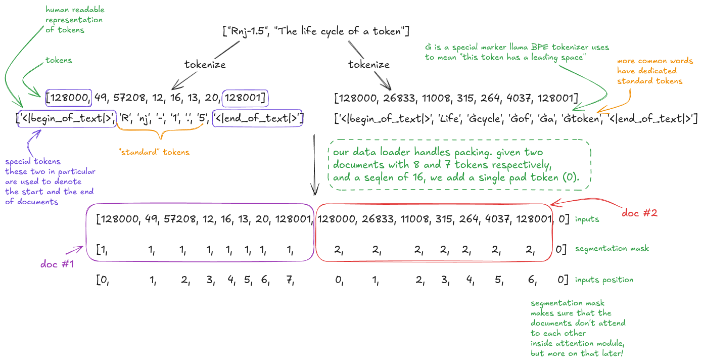
We tokenize the documents into sequences of integers, then pack the two documents into a single sequence.
Alongside the tokens, we construct two supporting structures:
- inputs positions - used by the positional embedding module (YaRN)
- segmentation mask - used in attention for masking
This is the preprocessing stage.
Next, we use the input tokens to index into the embedding table.
You can think of the embedding table as the vocabulary of the LLM.
This indexing operation converts our sequence of integers into a sequence of 16 4096-dim bf16 vectors:
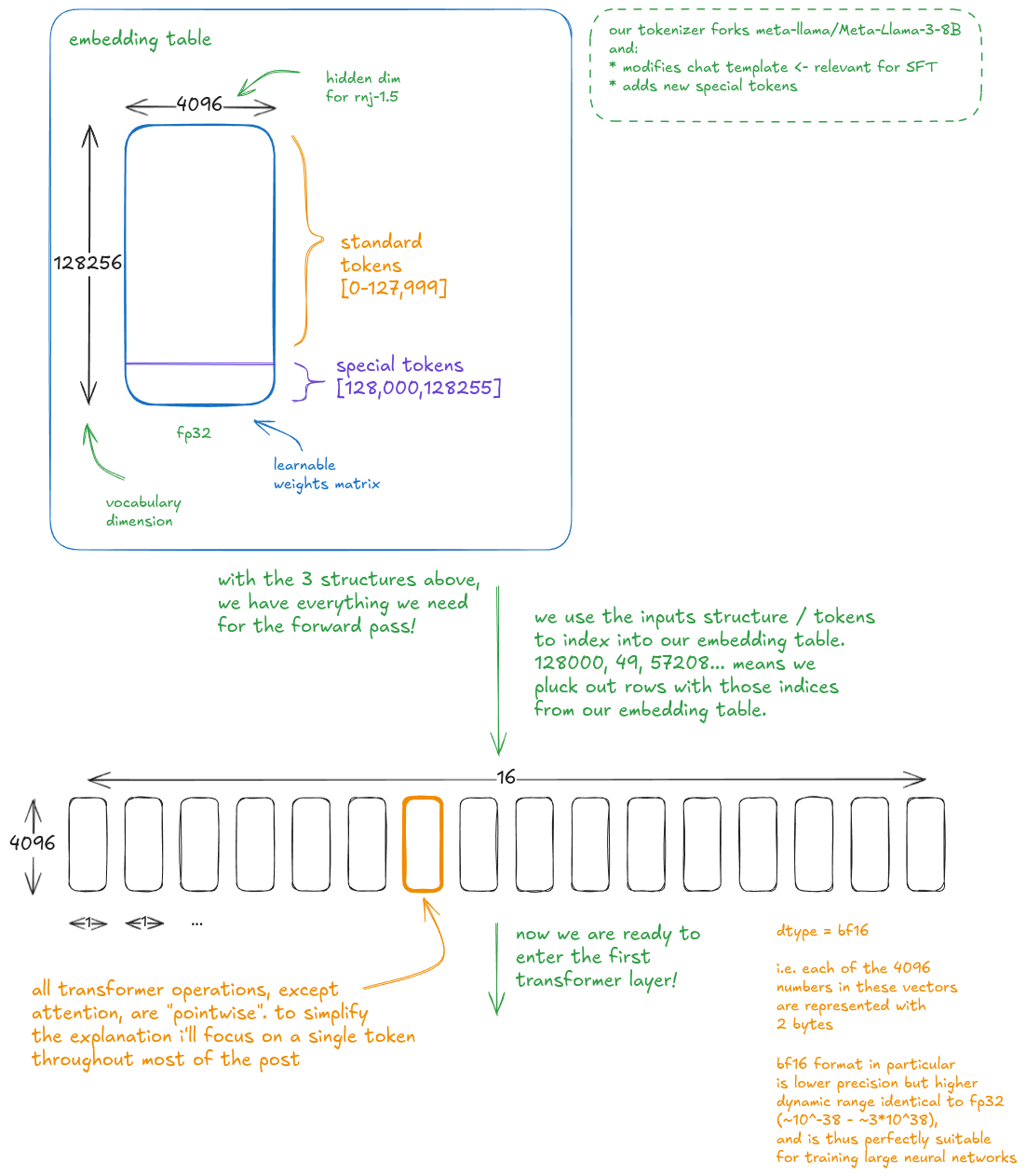
Special tokens don't naturally appear during tokenization - no text maps to token IDs >= 128,000. They're injected during training (and later used at inference) to improve performance (e.g. FIM, repo packing, etc.) or to enforce specific behaviors (e.g. end of generation / turn, tool calls).
Let's dig into FIM [3] (fill-in-the-middle) special tokens.
During (pre)training, we take a document, split it into prefix, middle (infix), and suffix, and construct a sequence of the form: <FIM_PRE> prefix <FIM_SUF> suffix <FIM_MID> middle. The model is trained to predict the middle given the prefix and suffix. This capability can then be leveraged at inference time.
For example, imagine using Rnj 1.5 as an autocomplete model in your favorite IDE. Your cursor naturally splits the code into a prefix and suffix, with the middle missing. By inserting FIM tokens and ending with <FIM_MID>, you prompt the model to generate a completion for the gap. These tokens help communicate intent to the model.
Tokenizer can easily be its own blog post, so I'll stop here.
Now we're ready to enter the first transformer layer.
Note that all transformer layers have (almost) the same structure, so I'll explain just one. In practice, we pass through 32 such layers - you can think of it as a for loop, but in Rnj 1.5 each layer has its own learnable weights.
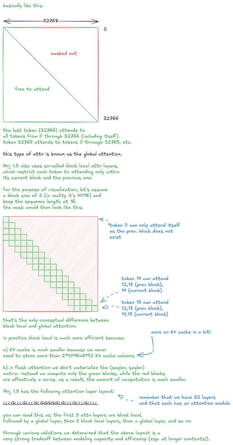
“almost” because Rnj-1.5 uses both block-local and global attention layers - the only difference is the mask. At a higher level of abstraction, the statement still holds. More on that in the attention section.
also note that some transformer implementations do weight sharing or partial weight sharing between layers (there are many variations) but here we're focusing on Rnj 1.5.
Let's do a forward pass through transformer blocks. Analyze the following carefully:
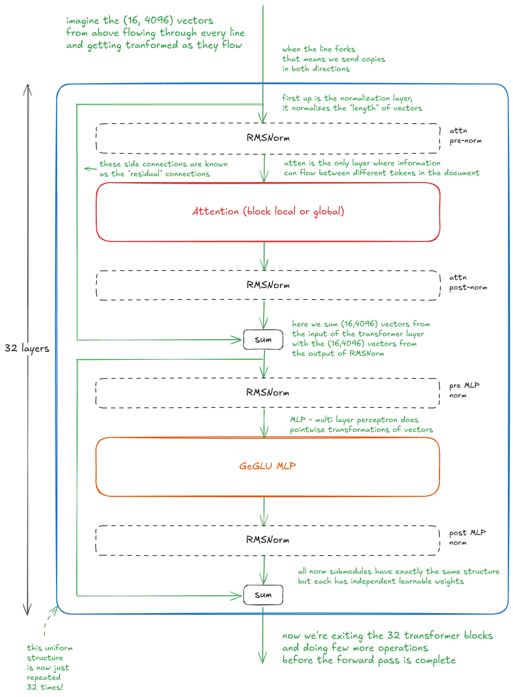
At a high level, the block consists of four RMSNorm submodules, an MLP, an attention module, two residual connections, and two sum operations. The residual connections simply carry forward copies of vectors from earlier in the block.
Importantly, all submodules operate on individual vectors, except for attention.
In practice, you'll find many variations of the transformer block. Design choices include the placement, type and number of normalization layers, the exact MLP structure (gated vs. non-gated, the choice of gating function, etc.), residual connections structure (identity, Attention Residuals [4], etc.), and especially the attention module.
Broadly, attention mechanisms are either quadratic (e.g. MLA [5], scaled dot-product attn, etc.) or linear (e.g. Kimi Linear [6]) in sequence length, each with trade-offs between modeling capacity (especially at long context) and efficiency.
Once the vectors exit the final transformer block, they're projected into a 128,256-dimensional space via a matrix multiplication. This produces logits, which are converted into a probability distribution via softmax. We sample from it during inference and use it in the cross-entropy loss during training.
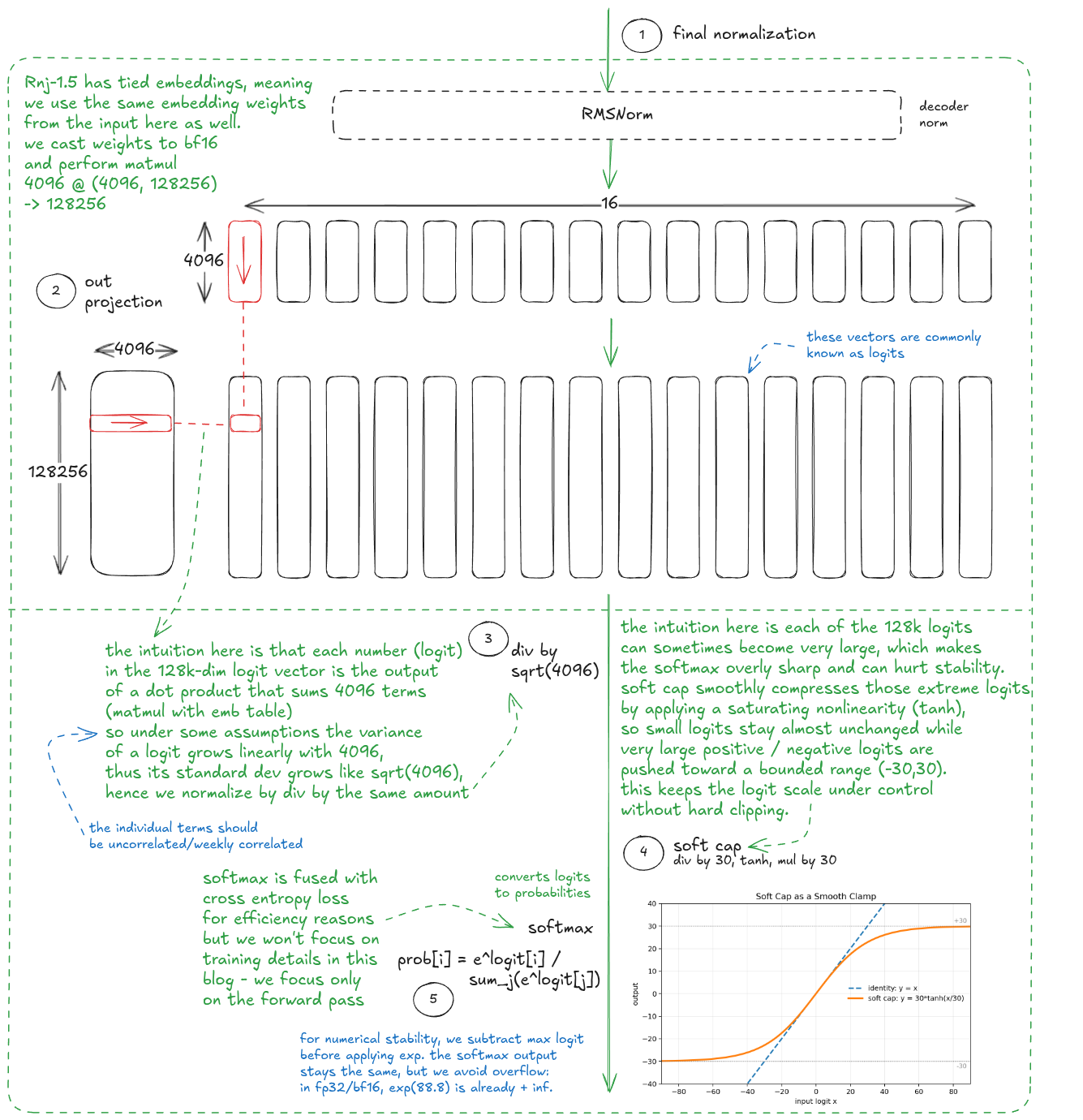
Next, let's dive into the individual sublayers. I'll go in reverse order this time, which conveniently takes us from the simplest to the most complex:
- RMSNorm (Root Mean Square Layer Normalization)
- GeGLU MLP (Multi-Layer Perceptron)
- Attention (Scaled Dot-Product Attention)
RMSNorm (Root Mean Square Layer Normalization)
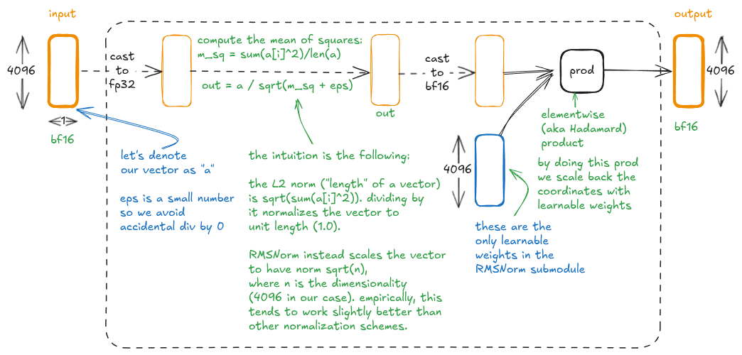
RMSNorm [7] is a normalization technique used to stabilize the training of deep neural networks.
As mentioned earlier, RMSNorm operates on individual vectors, so we'll focus on a single bf16 4096-dim vector (all others are processed in parallel in the same way). The output has the same shape and dtype:
GeGLU MLP (Multi-Layer Perceptron)
The MLP is a simple, pointwise feedforward neural network that is used to learn the non-linear relationships between the input and output vectors.
Our variant is GeGLU (GELU-gated linear unit [8]), where the gating mechanism uses GELU and takes the form W2 @ GELU(W0@X)*(W1@X):
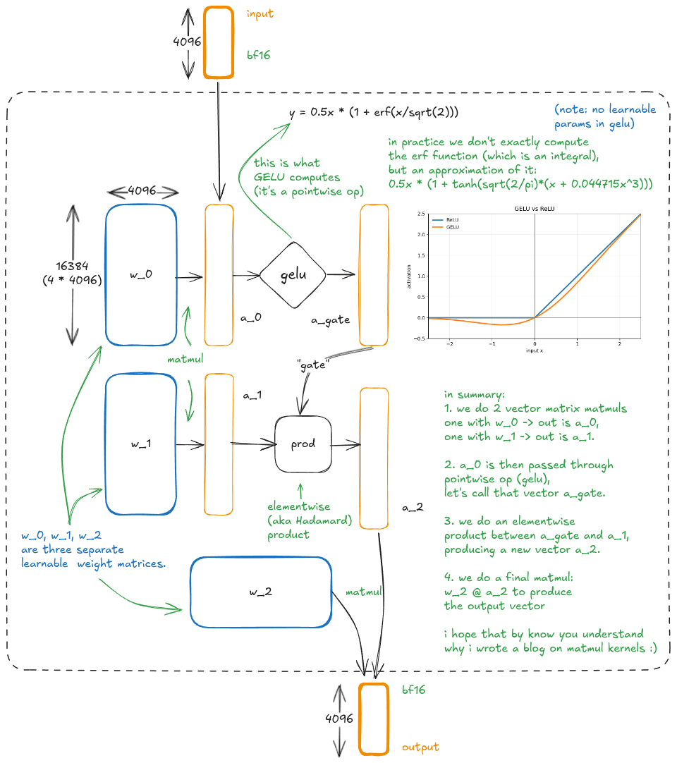
With ReLU, “gate” is more literal because the gating vector is nonnegative, so it only suppresses or scales features. With GELU, gating values can be negative, so the gate can also invert a feature's sign, which makes “gate” a looser historical term.
MHA (Multi-Head Attention)
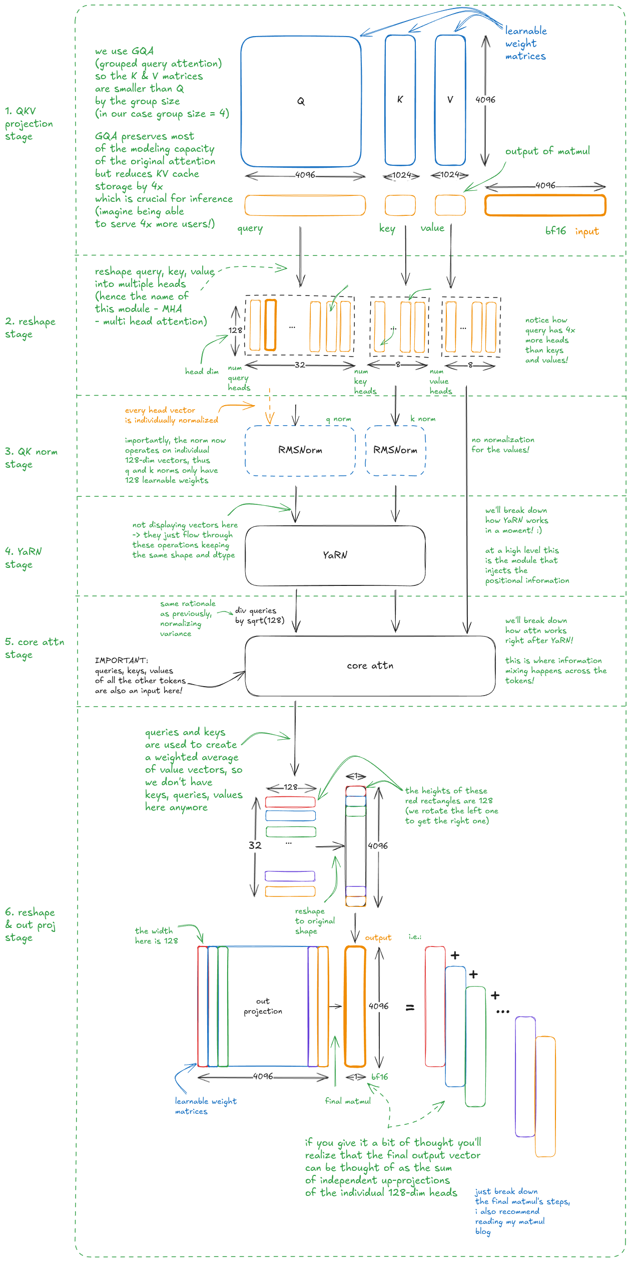
MHA is a self-attention mechanism used to model relationships between different tokens in a sequence. We use a special variant of MHA, called GQA, short for group query attention (the number of K/V heads is reduced compared to Q heads, hence multiple queries (group) attend to the same key).
First, I'll give the high level overview - then we'll dig into the two most interesting components: YaRN and core attention.
We start by mapping each vector independently into query, key, and value vectors. We then reshape them, normalize queries and keys, and apply YaRN (which injects positional information through rotation). Next comes core attention, which mixes information across positions. Finally, we apply a linear projection to produce the output.
Let's now focus on YaRN (Yet another RoPE extensioN).
YaRN
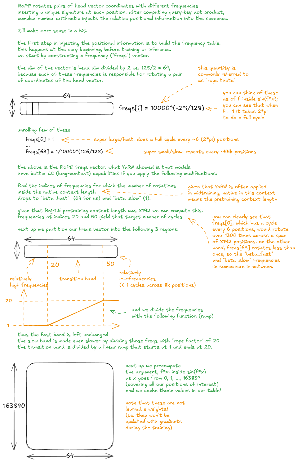
YaRN [9] modifies RoPE [10] (rotary position embeddings) in a clever way, that leads to better extrapolation to longer context lengths.
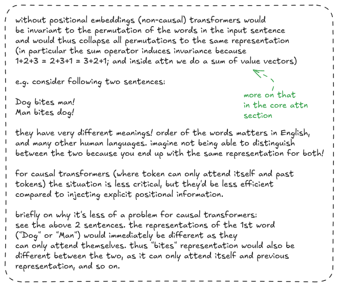
But why do we need positional embeddings in the first place?
Now that we understand the why, let's see how does RoPE work:
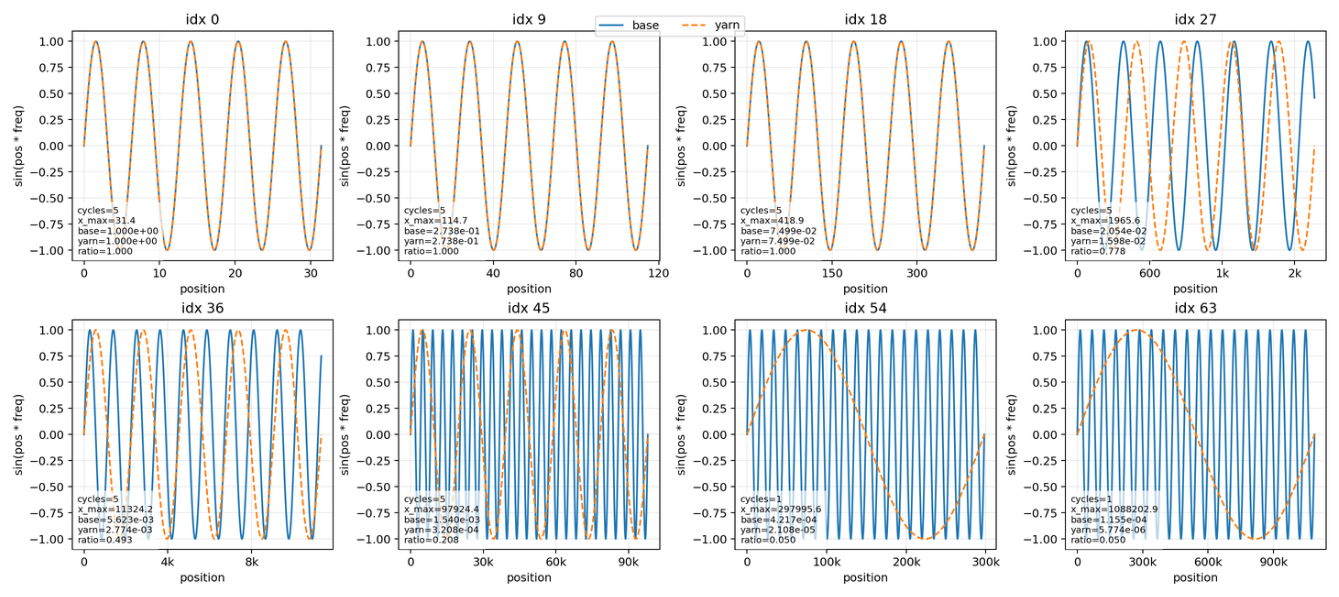
Here is a visualization showing how different YaRN frequencies behave. Notice that our slowest frequency does 1 cycle every 1.088M positions!
With this we're ready to see how positional embeddings are injected during the forward pass:
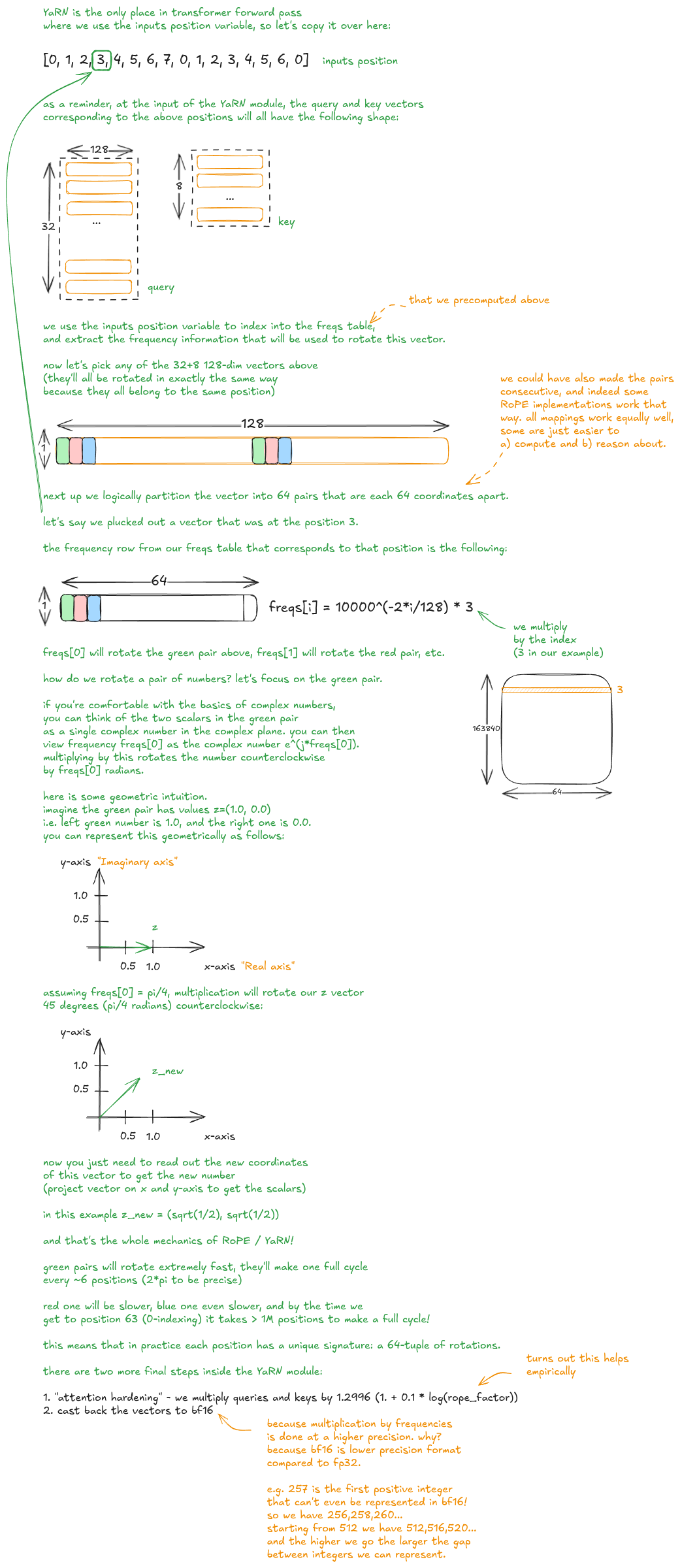
That wraps up the YaRN forward pass.
Now that we understand the mechanics of it you might still be wondering: how does YaRN encode relative positional information via pairwise coordinate rotations of the query and key vectors, followed by a dot product?
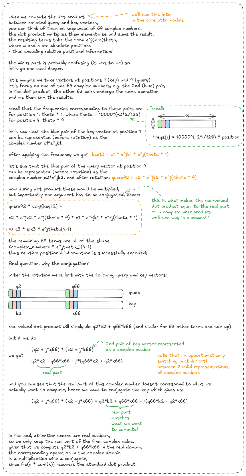
And that's all there is to RoPE/YaRN! :)
Core Attention
Finally, let’s analyze the core attention mechanism. In practice, we use FlashAttention, which deserves a separate blog post (I actually wrote one back in ’23, check it out [11]). Here, I’ll walk through vanilla attention.
Core attention is the mechanism that models relationships between tokens in a sequence. Take some time to analyze this:
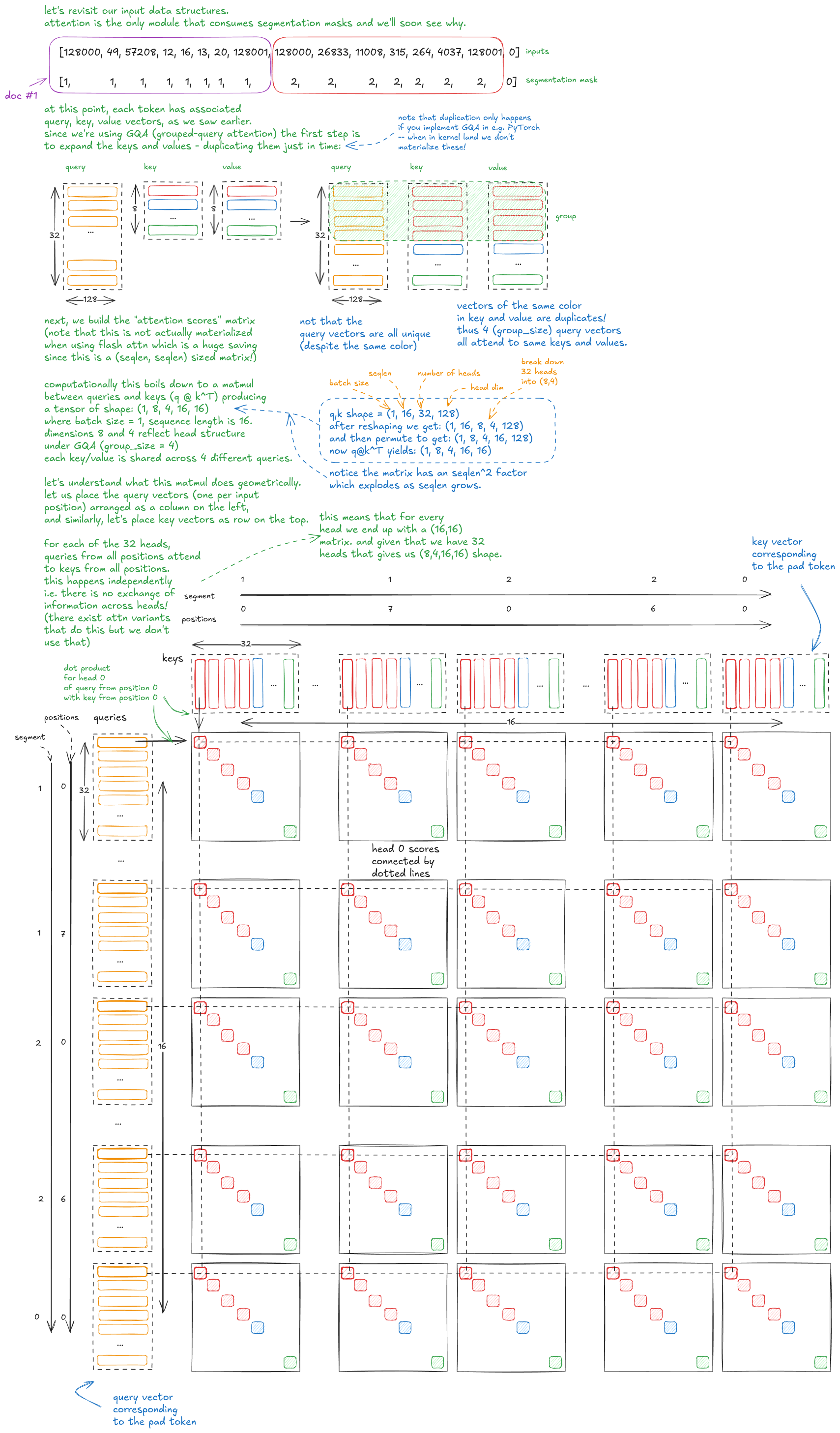
Now if we just stopped here we'd have a situation where:
- tokens from document 1 could attend to tokens from document 2 (and vice versa)
- token
icould attend to tokeni+1(future token) which breaks the causality
In order to prevent this we need to introduce masking!
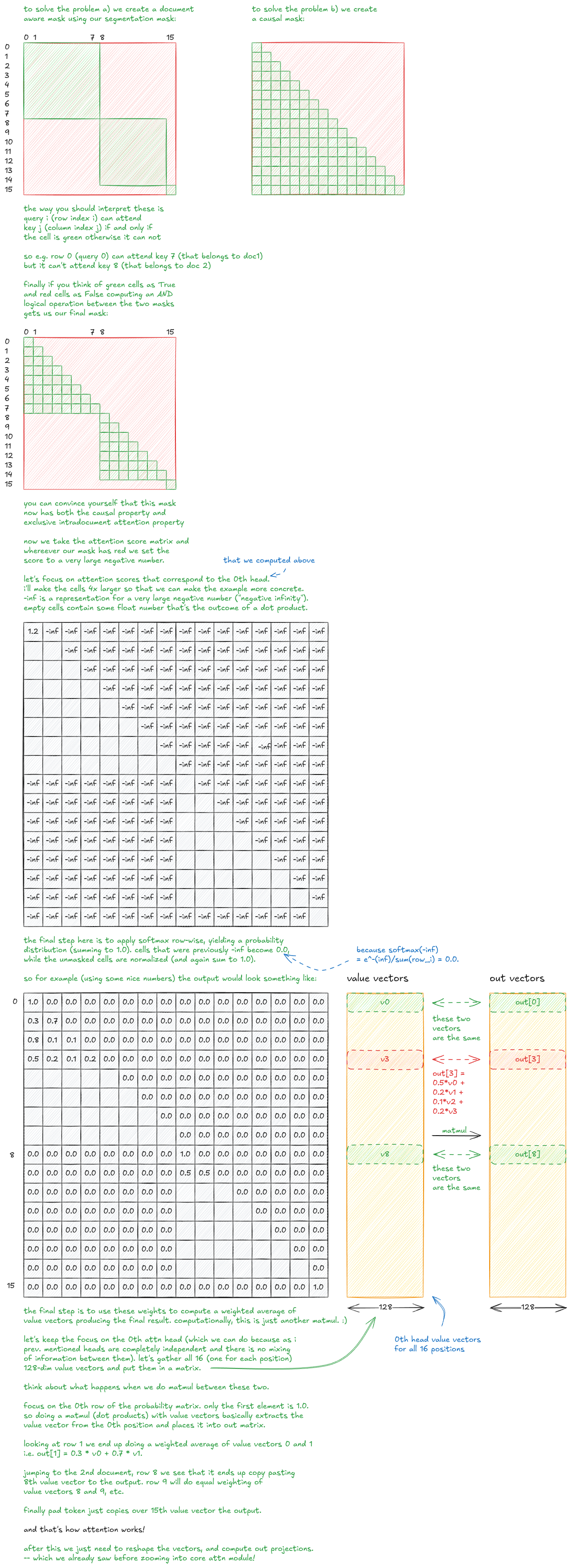
Now imagine our sequence length is 32,768 instead of 16. For simplicity, assume a single document with no padding. What would the mask look like?
Here’s another way to visualize the layout, focusing on tokens at positions 9,000 and 10,000:
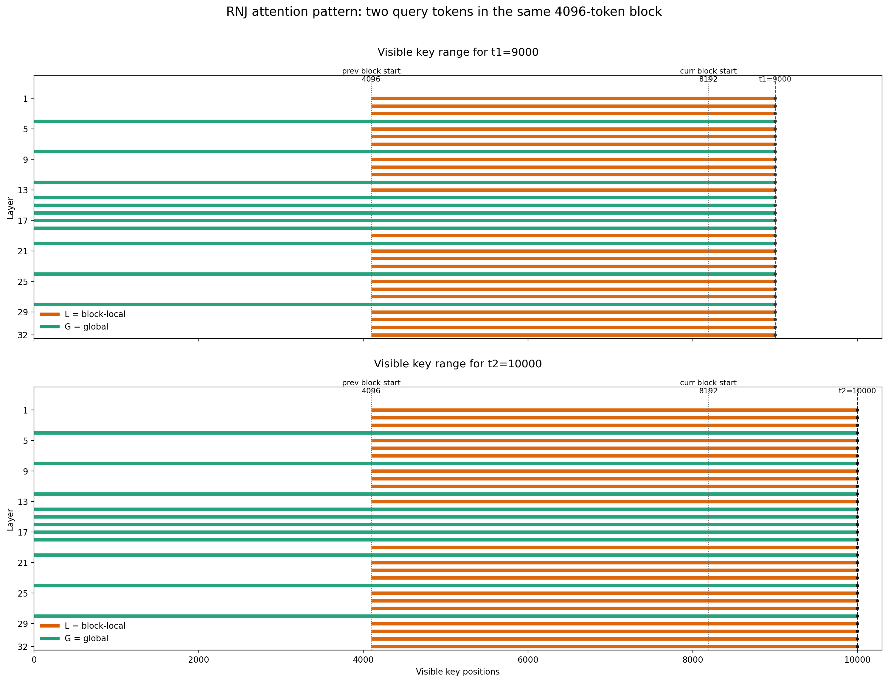
You can see that in most layers (block-local), these two tokens cannot attend to positions beyond 4,096. In the remaining eight layers (global), they can attend all the way back to position 0.
Transformer math
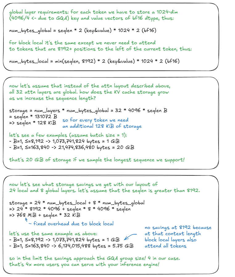
Finally, I want to briefly touch on the KV cache, as it’s an extremely important concept for understanding inference. So far, we’ve looked at the forward pass during training.
During inference, transformers are autoregressive - we generate one token at a time. It would be extremely inefficient to recompute the keys and values for all previous tokens at every step. Fortunately, there’s no need: in a causal transformer, they remain unchanged. Instead, we compute them once and store them in a cache.
Let’s go through the basic KV cache storage requirements:
Let's now also calculate how many learnable parameters Rnj 1.5 has. We just need to go through the architecture and account for all the learnable weights.
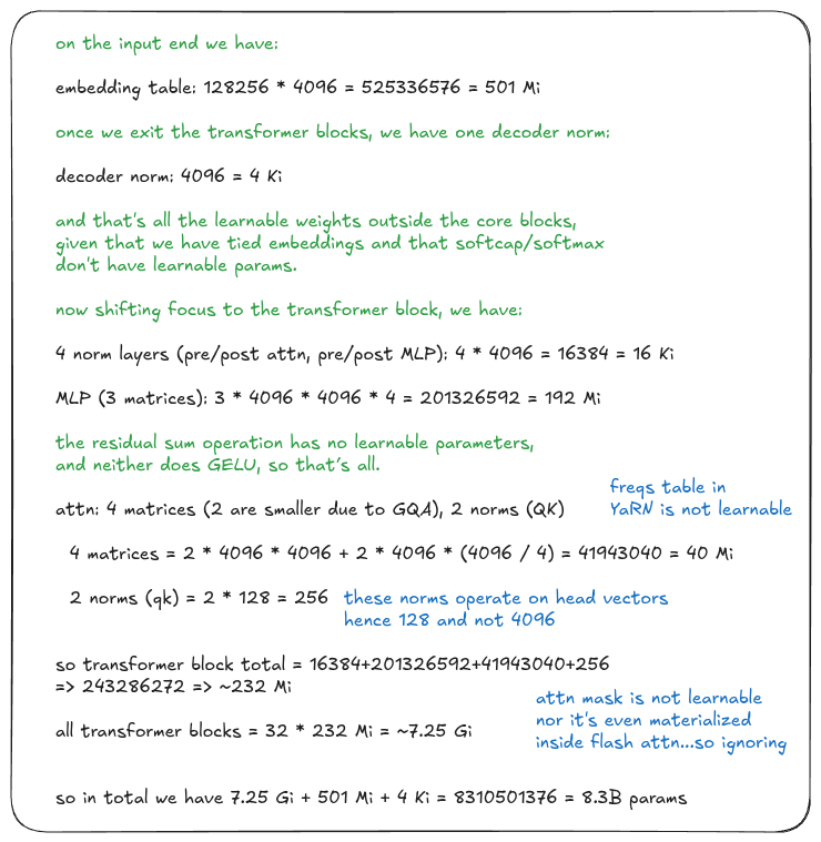
For quick mental math notice that you only need to account for 3 matrices inside MLP and 4 matrices inside attention and you can ignore everything else.
Let's now calculate how much compute (FLOPs) we need per token. This is extremely valuable when it comes to planning cluster sizing - more on that after this section.
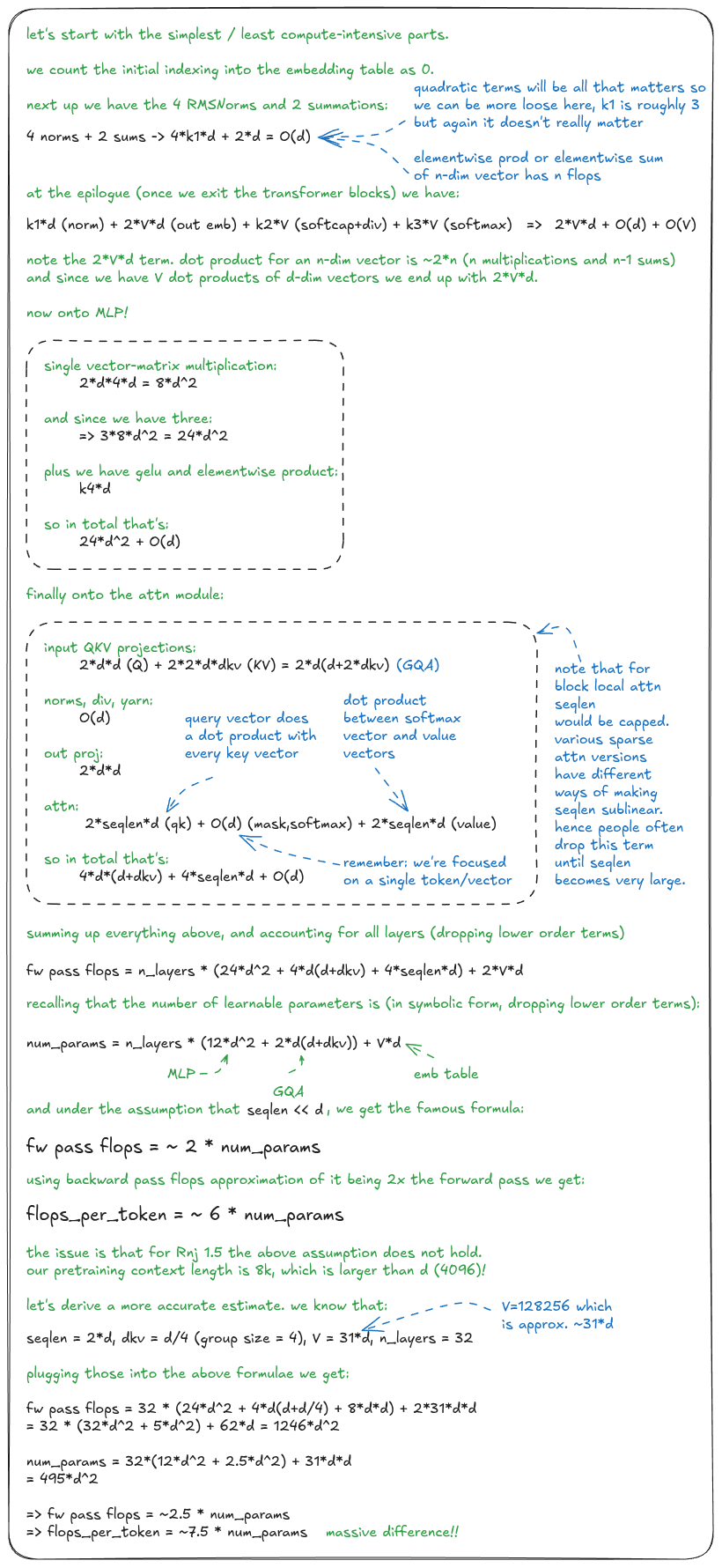
It's worth remembering the 6N formula. It's also worth remembering the setting under which it holds (i.e. seqlen << inner model dimension).
Finally let's see how we can use the above formula for cluster sizing:
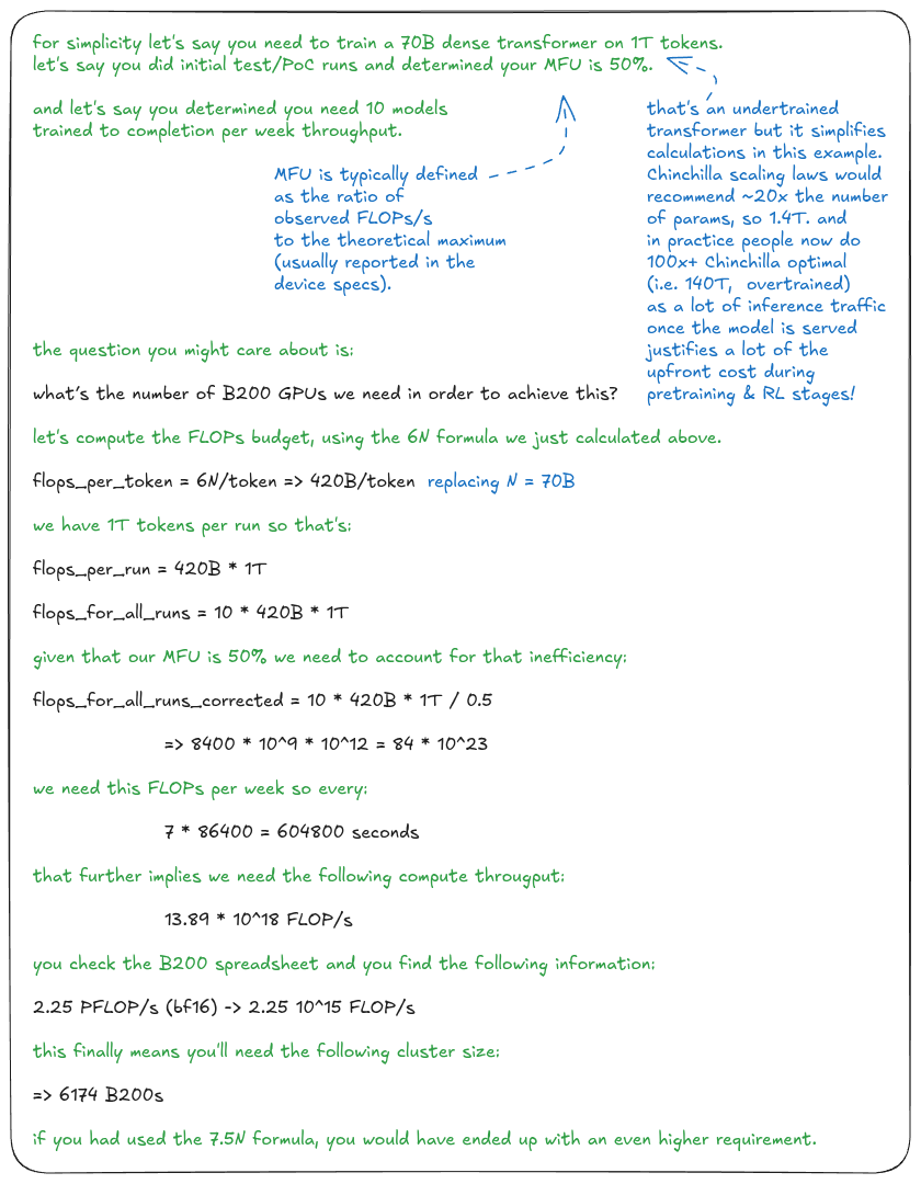
You now go to Masayoshi Son and ask for a $1B seed round.
Epilogue
We've seen how a single token flows through the transformer and how all the subcomponents work together.
We've explored YaRN and attention in depth, and derived some of the most important transformer formulas.
In upcoming posts, I'll dig deeper into MoE, Muon (the optimizer [12]), and several architectural innovations such as MLA (DeepSeek), MTP (multi-token prediction), and DSA (sparse attention [13]).
Get notified when I publish a new post.
References
- "Attention Is All You Need", https://arxiv.org/abs/1706.03762
- RNJ 1.0, https://essential.ai/research/rnj-1
- "Efficient Training of Language Models to Fill in the Middle", https://arxiv.org/abs/2207.14255
- "Attention Residual Learning", https://arxiv.org/abs/2603.15031
- "DeepSeek-V2: A Strong, Economical, and Efficient Mixture-of-Experts Language Model", https://arxiv.org/abs/2405.04434
- "Kimi Linear: An Expressive, Efficient Attention Architecture", https://arxiv.org/abs/2510.26692
- "Root Mean Square Layer Normalization", https://arxiv.org/abs/1910.07467
- "GLU Variants Improve Transformer", https://arxiv.org/abs/2002.05202
- "YaRN: Efficient Context Window Extension of Large Language Models", https://arxiv.org/abs/2309.00071
- "RoFormer: Enhanced Transformer with Rotary Position Embedding", https://arxiv.org/abs/2104.09864
- "Eli5 Flash Attention", https://gordicaleksa.medium.com/eli5-flash-attention-5c44017022ad
- Muon, https://kellerjordan.github.io/posts/muon/
- "Dissecting Sparsity in Large Language Models: Intrinsic Data-Aware Sparse Attention", https://arxiv.org/abs/2512.02556